The big O
Running code with small data sets can seem instantaneous, but when dealing with big data sets, the amount of computational resources an algorithm takes becomes vital. Programmers denote the resources taken for an algorithm with big ‘O’ notations, where n = size of data set.
You may see o, Ω & Θ in addition to O, which are all expressions of the asymptotic behavior of the function.
f(n) = O(g(n)) means that f doesn’t grow faster than g. g is an upper bound.
f(n) = o(g(n)) means that f grows strictly slower than g. g is an upper bound.
f(n) = Ω(g(n)) means that f doesn’t grow slower than g. g is a lower bound.
f(n) = Θ(g(n)) means that f grows as fast as g. g is a tight bound, both upper and lower.
These notations are approximate and algorithms are described in orders of O(1), or O(n²). Below is a graph charting the different notations:
Where this is relevant is in the order of operations taken for different algorithms and when to use them. For instance, with large data sets, algorithms like Merge Sort or Quicksort would generally be faster than Bubble Sort. There are more complexities to using sorting algorithms depending on whether you have enough memory, or type of cores, etc.
O(1)
Constant time: Remain constant regardless of n
Examples: Hashtable access, Push, Pop
O(log n)
Logarithmic time: If n doubles, the time complexity increases by a constant < n
Example: Binary search (dividing the search array length by half each operation)
O(n)
Linear time: Increases proportionate to n
Example: Linear search
O(n log n)
Linearithmic time: Increases at a multiple < n
Examples: Quicksort, Merge Sort
O(n²)
Quadratic time: Increases in proportion to n*n
Example: Bubble Sort
O(n!)
Factorial time: Increases in proportion to the factorial (1*2*3…*n)
Example: Solving Travelling Salesman Problem via brute force
Sorting Algorithms
Stability
In addition to computational complexity, stability is also a factor when deciding which algorithms to use. Stability simply means that the equal key values elements are preserved in their original order.
For instance:
5¹ 2 5² 1 6 → 1 2 5¹ 5² 6
Selection Sort
Selection Sort sorts an array by repeatedly finding the minimum element in the unsorted pile and swaps it for the first unsorted element and call that minimum element sorted. It stops when there are no unsorted elements.
for i = 1:n,
    k = i
    for j = i+1:n, if a[j] < a[k], k = j
    → invariant: a[k] smallest of a[i..n]
    swap a[i,k]
    → invariant: a[1..i] in final position
end

// code via toptal.com
It can be unstable, as when the first element 5¹ is swapped with 1 at the back:
5¹ 2 5² 1 6 → 1 2 5² 6 5¹ → 1 2 5² 5¹ 6
The run time is always quadratic, because it needs to go through all the elements in the array every single turn. You may think this means it should never be used, but because of the minimum number of swaps compared to other algorithms, it can be optimal when swapping has high computational cost.
Bubble Sort
Bubble Sort works by repeatedly swapping adjacent elements in they are in the wrong order.
Eg:
First pass: 5 1 4 2 → 1 5 4 2 → 1 4 5 2 → 1 4 2 5
Second pass: 1 4 2 5 → 1 4 2 5 → 1 2 4 5 → 1 2 4 5
for i = 1:n,
    swapped = false
    for j = n:i+1,
        if a[j] < a[j-1],
            swap a[j,j-1]
            swapped = true
    → invariant: a[1..i] in final position
    break if not swapped
end

// code via toptal.com
Bubble Sort has a quadratic run time, at a slightly higher overhead than Insertion Sort. At a campaign event back in 2007 at Google headquarters, when asked, “What is the most efficient way to sort a million 32-bit integers?”, Obama answered “I think the bubble sort would be the wrong way to go.” It fares better when the array is nearly sorted, taking O(n) time, but is still slower than Insertion Sort.
Insertion Sort
Insertion Sort iterates over the array, inserting the current element in the correct position of the previously iterated elements. It is similar to how we typically sort our hand of playing cards.
Eg:
2 1 6 3 → 1 2 6 3 → 1 2 6 3 → 1 2 3 6
for i = 2:n,
    for (k = i; k > 1 and a[k] < a[k-1]; k--)
        swap a[k,k-1]
    → invariant: a[1..i] is sorted
end

// code via toptal.com
Insertion Sort is terrible when elements are sorted in reverse order, taking O(n²) time. However, it’s in small arrays and nearly sorted arrays where it shines, taking only O(n) time when nearly sorted. Because it is stable and has a low overhead, it is often also used as the recursive base case for other sorting algorithms with high overhead, like merge sort or quick sort.
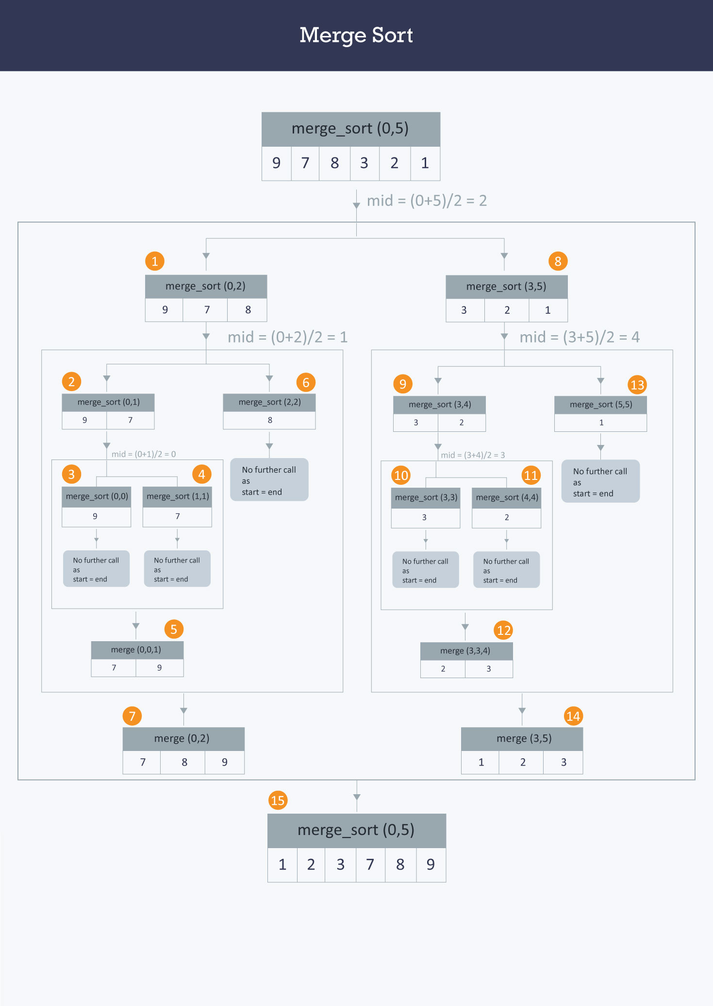
Merge Sort
Merge Sort is a Divide & Conquer algorithm. It divides the array in two halves, and then further break the half into halves until each sublist consists of a single element. It then merges the sublists into a sorted list.
# split in half
m = n / 2

# recursive sorts
sort a[1..m]
sort a[m+1..n]

# merge sorted sub-arrays using temp array
b = copy of a[1..m]
i = 1, j = m+1, k = 1
while i <= m and j <= n,
    a[k++] = (a[j] < b[i]) ? a[j++] : b[i++]
    → invariant: a[1..k] in final position
while i <= m,
    a[k++] = b[i++]
    → invariant: a[1..k] in final position

// code via toptal.com
As you might have guessed, the Divide & Conquer approach is useful for large arrays. Merge Sort is faster than the previous methods, taking Θ(n log n) time. It is predictable as well, taking 0.5 log (n) and log (n) comparisons and between log (n) and 1.5 log (n) swaps per element. It is the algorithm of choice because of its stability, simple implementation, and the fact that it does not require random access to data. However, it requires Θ(n) extra space for arrays, but only Θ(log n) for linked lists.
Quick Sort
Quick Sort is a Divide & Conquer algorithm which is similar to Selection Sort. Quick Sort divides a large array into two smaller sub-arrays from the pivot element and recursively sort the sub-arrays.
The steps are (visualized below):
1. Pick an element from the array.
2. Partitioning: reorder the array so that elements pivot value goes after it. (Equal values may be placed before or after, thereby making it unstable.)
3. Recursively apply the above steps to the sub-array of smaller elements and larger elements separately.

_# choose pivot_
swap a[1,rand(1,n)]

_# 2-way partition_
k = 1
for i = 2:n, if a[i] < a[1], swap a[++k,i]
swap a[1,k]
_→ invariant: a[1..k-1] < a[k] <= a[k+1..n]_

_# recursive sorts_
sort a[1..k-1]
sort a[k+1,n]

// code via toptal.com
Quick Sort takes typically O(n log n) time, and O(n²) time on rare occasions. It is robust and has low overhead when implemented properly (a 3-way partition should be used instead of the example above). It fulfills a general purpose role when stability is not required and extra space is not a problem.
When both sub-sorts are performed recursively, quick sort requires O(n) extra space in the worst case scenario, but can be optimized to use O(log n) extra space instead with optimization, by switching to a simpler algorithms for shorter sub-arrays.
For other optimization, visit: https://yourbasic.org/golang/quicksort-optimizations/
Sorting Algorithm Cheat Sheet
| Algorithm | Best-case | Worst-case | Average-case | Space Complexity | Stable? |
| Merge Sort | O(n log n) | Ω(n log n) | O(n) | O(n) | Yes |
| Insertion Sort | O(n) | Ω(n²) | O(n²) | O(1) | Yes |
| Bubble Sort | O(n) | Ω(n²) | O(n²) | O(1) | Yes |
| Quicksort | O(n log n) | Ω(n²) | O(n log n) | log n best, n avg | Usually not |
| Heapsort | O(n log n) | Ω(n log n) | O(n log n) | O(1) | No |
| Counting Sort | O(k + n) | Ω(k + n) | O(k + n) | O(k+1) | Yes |
